
Index function can be used to get a reference of cell from an Array for required or matching value. It’s basic use require three parameters. We’re going to describe the function with example.
Step#1:
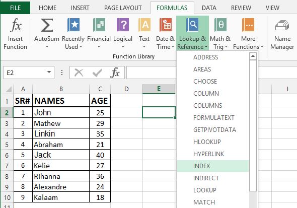
We’re going to use the following list in excel to use the index function:

Index function’s structure is:
= INDEX(array, rownum,[columnnum])
Where ‘array’ is the area of values from with the reference cell will be returned.
‘rownum’ is the index number of row from where the reference cell value will be reflected.
‘[columnnum]’ is the index number of column. By default, its value is 1. If array contains multiple columns (i-e: A,B,C), you can pass the index number accordingly to reflect the value. It’s optional, so that if you’ll not pass it, it’ll be considered as 1.
Step#2:
We’ll now apply the formula on the array. So take your focus to another cell, go to formula tab, click ‘lookup and reference’ and select index.
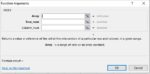
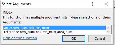
Popup window will appear, select first and press ‘OK’.
STEP#3:
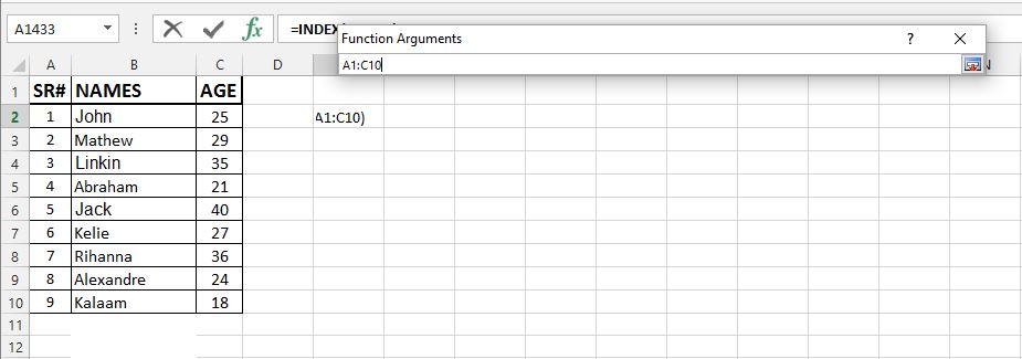
Windows Dialog will appear for parameter input for formula. In array, press the button next to input text field, and go to the sheet and select the array.
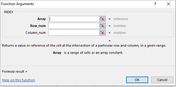
After selection of array, press that button again.
Step # 4:
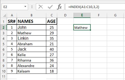
In the second text field, pass the row number that can be 1, 2, 3 and upto how many rows your array hold.
In the third text field, pass the column number, if your array holds multiple column area.
And Press ‘OK’. It’ll apply the formula to the cell you’re focusing. Now that cell will reflect the value of reference cell, i-e: value of row number 3, column number 2 from you array.
Step#5
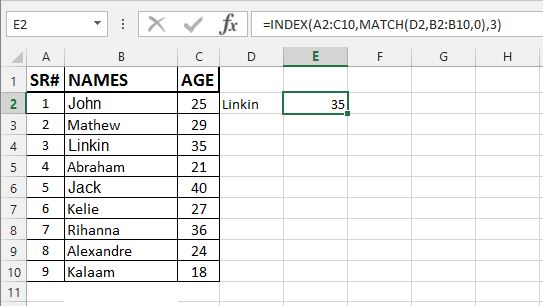
You can also use condition for to reflect required value from an array with the use of ‘MATCH’ function. You can apply match function in the replacement of row number that will check if specified value matched the row in array.
We will use the value of cell D2 to match in array and return the age of that person.
So, repeating the above first 3 steps, we’ll insert the formula in the ROW text field.
MATCH formula also required three parameters:
Lookup Value: Value that you need to match. We’ll give the reference D2 cell here.
Lookup Array: Array from where you want to match the Lookup value. We want to match the name, so we’ll pass B2:B10 array here.
MatchType: it’s the type of match that is less than, greater than or equal to. -1, 0, 1 are the keys to represent the types.
So, we’ll write “MATCH(D2, B2:B10,0)” in the Row Text field and 3 in the Column Text field, so it’ll give the value of Age.
This is the way to get matching values from the larger array in your worksheet. If you have any query regarding this tutorial, write down in the comments section.