How to Create Lookup Formulae with Multiple Criteria in Excel 2013
If you often find yourself dealing with large spreadsheets, learning how to create lookup formulae with multiple criteria in Excel 2013 will save you a lot of time. Once you learn how to create lookup formulae with multiple criteria in Excel 2013, you will not waste time manually searching through tables trying to find relevant information. Unlike VLOOKUP and HLOOK UP, using an array formula allows you to select multiple criteria to search based on.
Step 1: Launch Word 2013
Step 2: Open a document where you wish to create a lookup formula
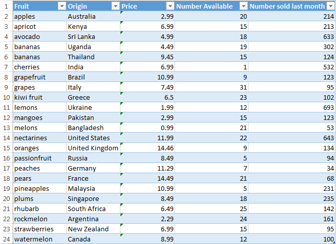
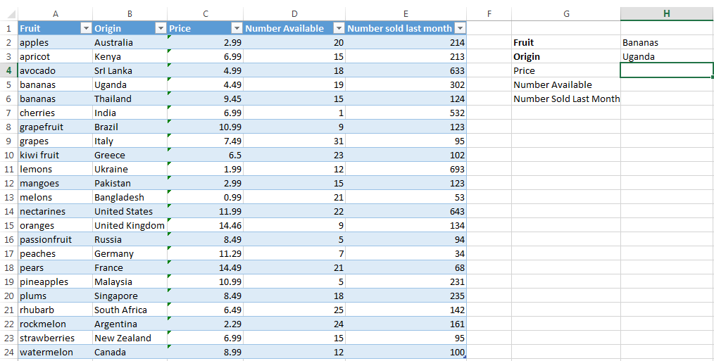
Step 3: In this example, want to search for the price of bananas produced in Uganda. We enter in the necessary data as shown in cells G2:H6. Click on cell H4
Step 4: Select the Formulas tab
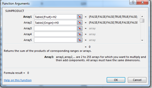
Step 5: Click on Math & Trig button under the Function Library and select SUMPRODUCT
Step 6: Enter in each area you are searching in and the cell containing the particular value you are searching for. For instance, in the first column titled Fruits, we are searching for “bananas” which is located in H2. Once you have entered all the conditions, click OK
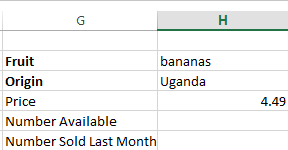
Step 7: The corresponding price will appear. You can repeat these steps to find the Number Available and the Number Sold Last Month


