
This tip describes a quick method to randomize a list. It’s like shuffling a deck of cards, where each row is a card.
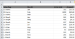
Figure 165-1 shows a two-column list, arranged alphabetically by column A. The goal is to arrange the rows in random order.

Figure 165-1: This alphabetized list will be randomly arranged.
1. In cell C1, enter the column heading Random.
2. In cell C2, enter this formula:
=RAND()
On the Insert tab, the galleries include items that are designed to coordinate with the overall look of your document. You can use these galleries to insert tables, headers, footers, lists, cover pages, and other document building blocks. When you create pictures, charts, or diagrams, they also coordinate with your current document look.
You can easily change the formatting of selected text in the document text by choosing a look for the selected text from the Quick Styles gallery on the Home tab. You can also format text directly by using the other controls on the Home tab. Most controls offer a choice of using the look from the current theme or using a format that you specify directly.
To change the overall look of your document, choose new Theme elements on the Page Layout tab. To change the looks available in the Quick Style gallery, use the Change Current Quick Style Set command. Both the Themes gallery and the Quick Styles gallery provide reset commands so that you can always restore the look of your document to the original contained in your current template.
3. Copy C2 down the column to accommodate the number of rows in the list.
4. Activate any cell in column C and choose Home➜Editing➜Sort & Filter➜Sort Smallest to Largest (or, right-click and choose the Sort command on the shortcut menu).
To get a different random configuration, press F9 to generate new random numbers and then sort again. Figure 165-2 shows the randomized list.

Figure 165-2: The list after being randomized.
Filling the Gaps in a Report
When you import data, you can end up with a worksheet that looks something like the one shown in Figure 166-1. This type of report formatting is common. As you can see, an entry in column A applies to several rows of data. If you sort this type of list, the missing data messes things up, and you can no longer tell who sold what when.

Figure 166-1: This report contains gaps in the Sales Rep column.
If your list is small, you can enter the missing cell values manually or by using a series of Home➜Editing➜Fill➜Down commands (or its Ctrl+D shortcut). But if you have a large list that’s in this format, you need a better way of filling in those cell values. Here’s how:
1. Select the range that has the gaps (A3:A14, in this example).
2. Choose Home➜Editing➜Find & Select➜Go to Special to display the Go To Special dialog box.

3. In the Go To Special dialog box, select the Blanks option and click OK. This action selects the blank cells in the original selection.

4. On the Formula bar, type an equal sign (=) followed by the address of the first cell with an entry in the column (=A3, in this example) and press Ctrl+Enter.
5. Reselect the original range and press Ctrl+C to copy the selection.
6. Choose Home➜Clipboard➜Paste➜Paste Values to convert the formulas to values.
After you complete these steps, the gaps are filled in with the correct information, and your worksheet looks similar to the one shown in Figure 166-2. Now it’s a more traditional list, and you can do whatever you like with it — including sorting.

Figure 166-2: The gaps are gone, and this list can now be sorted.