How to use Conditional Formatting in Excel 2013
Conditional formatting is a useful feature that has been inserted into Excel 2013. If you learn how to use conditional formatting in Excel 2013, you will be able to sort out your data with unprecedented ease. This feature allows you to filter out data according to your specifications and marking different categories of your data using different formatting techniques. In this guide, we will walk you through how to use conditional formatting in Excel 2013 so that you can not just sort out your data but also make it look great.
Step 1: Launch Excel 2013
Step 2: Open a document with data which you wish to use conditional formatting on

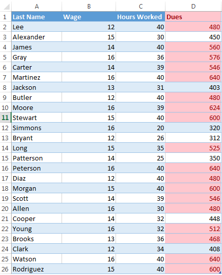
Step 3: If you want to add conditional formatting to every person who has dues greater than 450, select all the values in the entire dues column
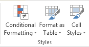
Step 4: Click on the Home tab
![]()
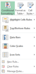
Step 5: Click on Conditional Formatting in the Styles section
Step 6: You can choose from a range of different filters in the Conditional Formatting dropdown menu

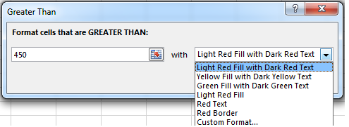
Step 7: Click on Highlight Cell Rules and Greater Than… Enter in the number and the formatting style you want and then click OK
Step 8: Your data will be formatted according to the condition specified
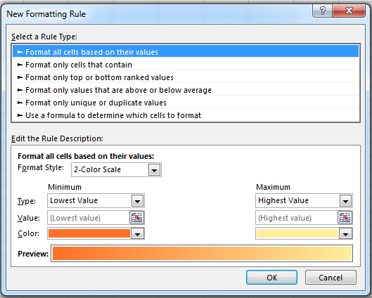
Step 9: You can also set various formatting rules by selecting New Rule… under the Conditional Formatting dropdown menu. Once set, these will continue to apply to all changes you make in your spreadsheet