
How to Create a PivotTable in Excel 2013
PivotTables are a great way to summarize your data. Many people shy away from using them because they don’t know how to create a PivotTable in Excel 2013. This step-by-step guide on how to create a PivotTable in Excel 2013 will help you make use of this great feature that Excel 2013 has to offer.
Step 1: Launch Excel 2013
Step 2: Open a document in which you wish to create a PivotTable
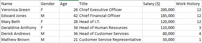
Step 3: Select a cell anywhere in the list of data which you wish to analyze
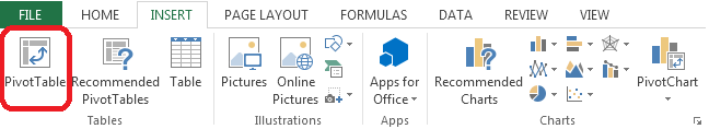
Step 4: Click on the Insert tab
![]()
Step 5: Click on Pivot Table in the Table section
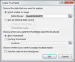
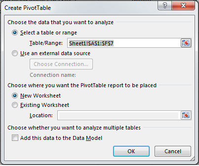
Step 6: In the PivotTable dialogue box that appears, adjust whatever cells you wish to include in your data. You can also choose whether you wish to add the PivotTable in the existing Workbook or in a new Workbook in the same document. When you have finalized your option, click OK and Excel will create your PivotTable
Step 7: Once the PivotTable is created, you can use the PivotTable Fields section that appears on the right of your page to decide which fields to add to your report
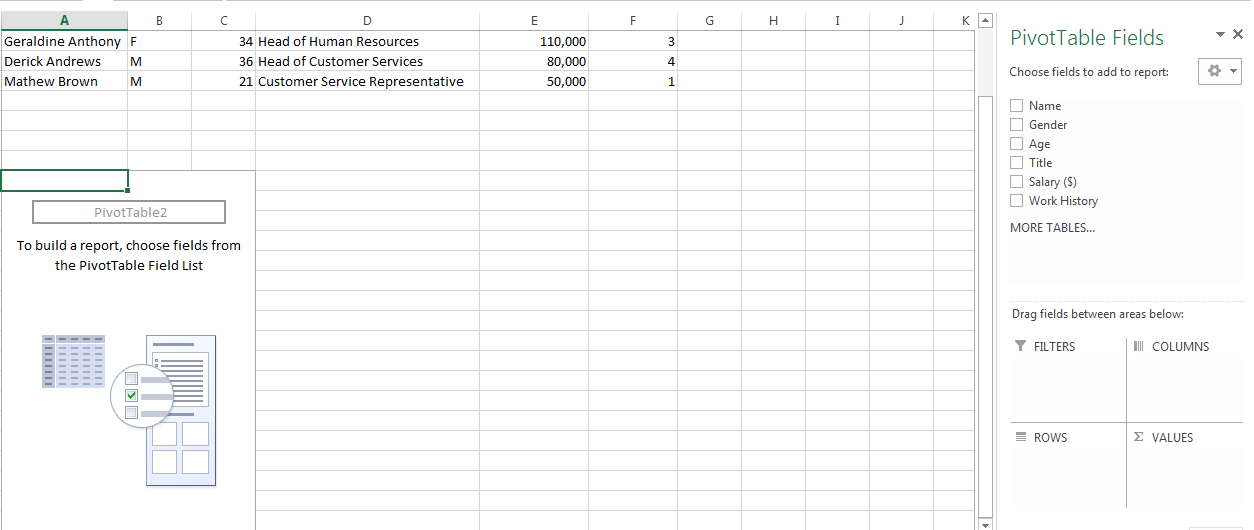
Step 8: As soon as you have added a particular field to your report, you have to assign a field list to that field. You can do this by dragging the field name into one of the four field list options on the PivotTable Fields menu towards the right. You can choose between FILTERS, COLUMNS, ROWS and VALUES
