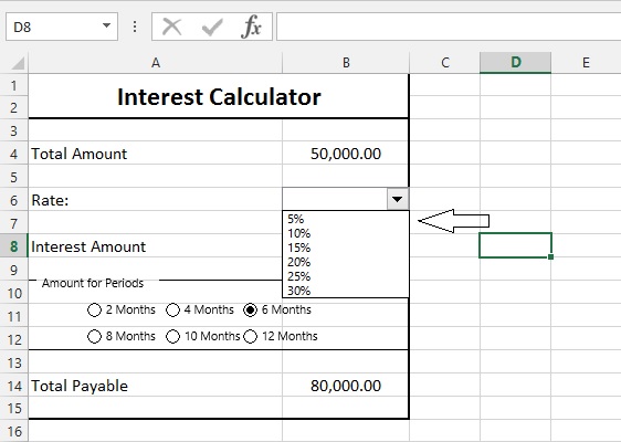
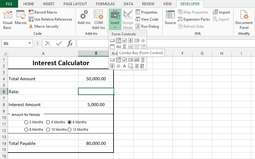
In this tutorial, we’ll show you how to use Combo Box form control in your excel sheet. We’ll be using Interest Calculator for this purpose, as shown below:
Step #1:
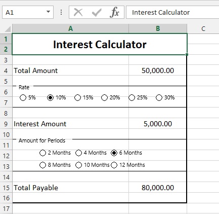
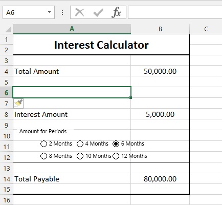
We’ll replace “Rate group box” with Combo Box. So, we’ll select Group box and press ‘Del’ button. Then, press ctrl and click on Radio Buttons to select them and press ‘del’. we’ll remove the rows 6 & 7 and Add one new row.
Step #2:
We’ll insert the Combo Box in B6 box. For that we need to insert Combo Box from Insert in Developers Option.
Step #3:
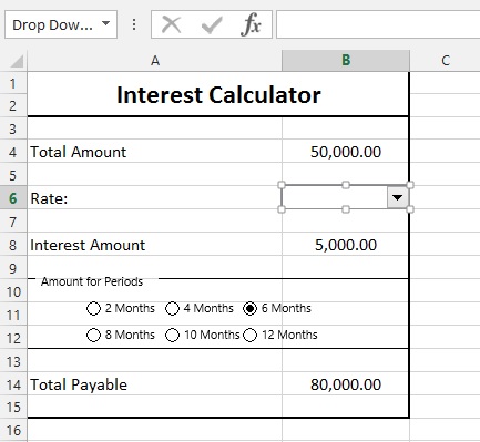
Press alt and, Click and drag in B6 to draw Combo Box.
Step #4:
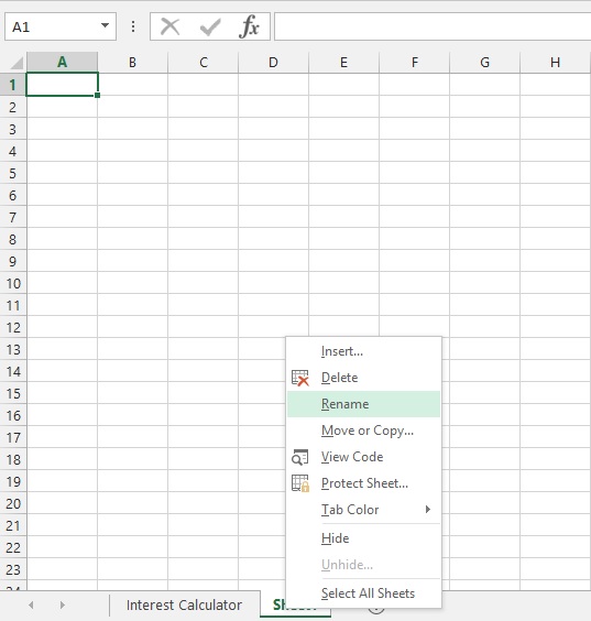
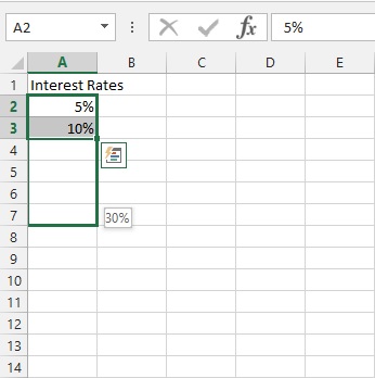
To add list of values, we need to list all the value on other sheet. And use that range in Combo Box. So, we’ll create new Sheet with the name “Data” and list all the values of interest rates.
We’ll enter two values with the difference of 5%. Select these two values and drag down to 5 cells. Excel will detect the difference and fill the values with the difference of 5% in each cell increasingly.
Step #5:
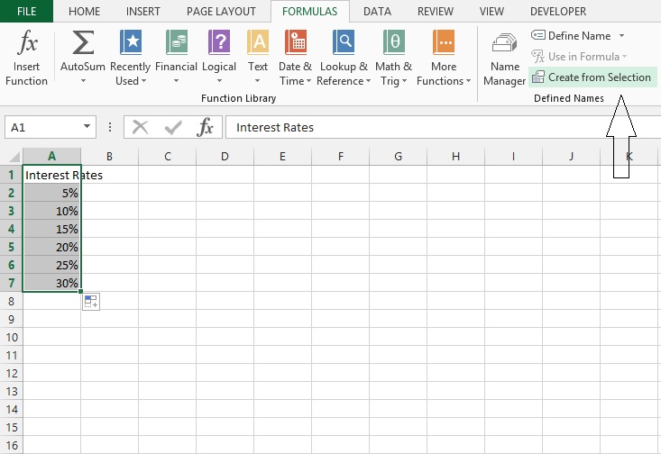
It’s best practice to define name for ranges to select them. So, We’ll select the cell ranges with values and go to “FORMULAS” ribbon tab. And select “Create from Selection”.
It’ll pop out a dialog box to give you options to select naming box for the range.
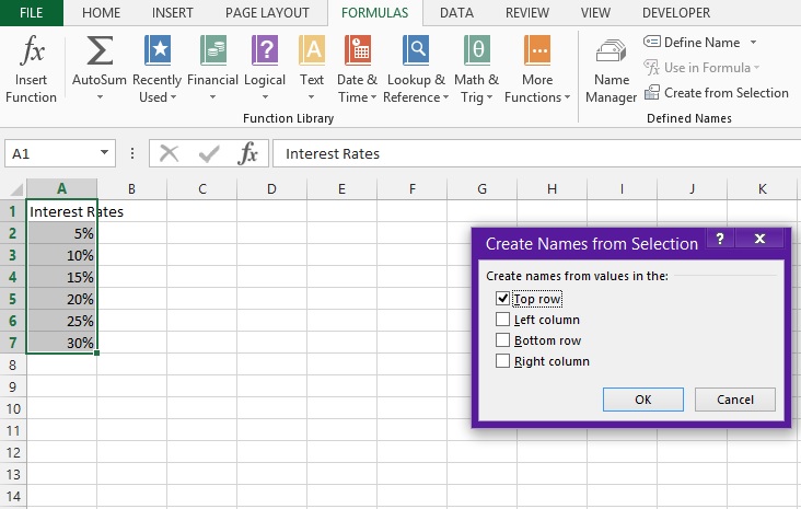
We have name to define range in the top row. So we’ll select “Top row” and select Press OK.
Step #6:
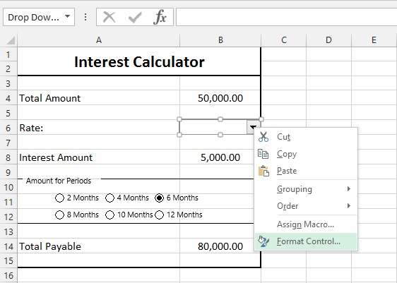
Now we have a defined name for the values of interest Rate. We’ll go to “Interest Calculator” Sheet. Select Combo Box and go to Format Control.
It’ll give you dialog box to insert range of cells for the values. We’ll insert the name defined for values.
I.e.: Interest_Rates
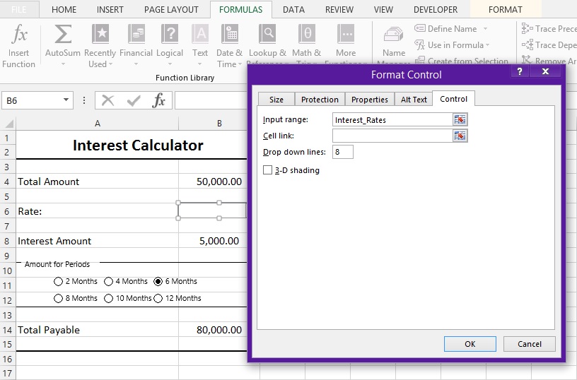
Press OK. Click on some other cell to remove selection focus of Combo Box. And then Check the Drop Down List, you’ll see all the values of range entered on “Data” Sheet.